Interpreting model results

After calling interlace.fit(), you receive a CrossedLMEResult object. This page explains what each part of the output means and how to use it to draw conclusions from your model.

Throughout this page we use a running example: exam scores modelled as a function of hours studied and prior GPA, with students and schools as crossed grouping factors.

import numpy as np
import pandas as pd
import interlace

rng = np.random.default_rng(42)
n = 300

df = pd.DataFrame({
    "score":         60 + rng.normal(0, 8, n),
    "hours_studied": rng.uniform(0, 10, n),
    "prior_gpa":     rng.uniform(2.0, 4.0, n),
    "student_id":    [f"s{i}"   for i in rng.integers(1, 31, n)],
    "school_id":     [f"sch{i}" for i in rng.integers(1, 11, n)],
})

result = interlace.fit(
    "score ~ hours_studied + prior_gpa",
    data=df,
    groups=["student_id", "school_id"],
)

/tmp/ipykernel_2509/4095886218.py:16: UserWarning: boundary (singular) fit: see help(interlace.isSingular)

---

Fixed effects

Fixed effects capture the population-level relationships between predictors and the outcome, controlling for the grouping structure.

The result exposes four attributes for fixed-effect inference:

Attribute	Contents
fe_params	Coefficient estimates (pd.Series)
fe_bse	Standard errors
fe_pvalues	Two-sided p-values (normal approximation)
fe_conf_int	95% confidence intervals (pd.DataFrame, columns [0.025, 0.975])

Reading the coefficients

fe_params is a pandas.Series indexed by term name. Each coefficient is the expected change in the outcome per unit increase in the predictor, holding grouping structure constant — i.e., the within-group effect.

result.fe_params

Intercept        60.454607
hours_studied     0.032509
prior_gpa        -0.322930
dtype: float64

Standard errors and inference

Standard errors in fe_bse account for the clustering: they are derived from the fixed-effect covariance matrix fe_cov = scale * (X'Ω⁻¹X)⁻¹, where X is the fixed-effect design matrix (one row per observation, one column per predictor including the intercept) and Ω is the marginal covariance matrix of the response that encodes the random effect structure. This is why they are typically larger than OLS standard errors on the same data — the effective sample size is reduced by the grouping.

A convenient summary table:

pd.DataFrame({
    "estimate": result.fe_params,
    "se":       result.fe_bse,
    "p":        result.fe_pvalues,
    "ci_lo":    result.fe_conf_int.iloc[:, 0],
    "ci_hi":    result.fe_conf_int.iloc[:, 1],
})

	estimate	se	p	ci_lo	ci_hi
Intercept	60.454607	2.446897	0.000000	55.658688	65.250526
hours_studied	0.032509	0.149269	0.827601	-0.260059	0.325077
prior_gpa	-0.322930	0.714485	0.651300	-1.723321	1.077460

P-values use a normal approximation (z-test), which is appropriate for large samples. For small samples with few groups, consider using likelihood-ratio tests or parametric bootstrap instead.

Comparing models with different fixed structures

To test whether a predictor improves fit, refit with method="ML" (not REML) and compare log-likelihoods. Use REML (the default) for your final reported estimates; use ML only for likelihood-ratio tests comparing fixed structures. See Concepts: REML for the reason.

from scipy.stats import chi2

m1 = interlace.fit("score ~ hours_studied",              data=df, groups=["student_id", "school_id"], method="ML")
m2 = interlace.fit("score ~ hours_studied + prior_gpa", data=df, groups=["student_id", "school_id"], method="ML")

lr_stat = 2 * (m2.llf - m1.llf)
df_diff = 1  # one extra parameter in m2
p_value = chi2.sf(lr_stat, df=df_diff)

print(f"LR statistic: {lr_stat:.3f}  (df={df_diff})")
print(f"p-value:      {p_value:.4f}")

LR statistic: 0.210  (df=1)
p-value:      0.6470

/tmp/ipykernel_2509/2957097658.py:3: UserWarning: boundary (singular) fit: see help(interlace.isSingular)
/tmp/ipykernel_2509/2957097658.py:4: UserWarning: boundary (singular) fit: see help(interlace.isSingular)

---

Variance components

Variance components quantify how much variability in the outcome is attributable to each grouping factor and to residual within-group noise.

Reading variance components

print("Between-group variances:")
for g, v in result.variance_components.items():
    print(f"  {g}: σ² = {v:.3f}  (σ ≈ {v**0.5:.2f} score points)")

print(f"\nResidual variance (scale): σ² = {result.scale:.3f}  (σ ≈ {result.scale**0.5:.2f} score points)")

Between-group variances:
  student_id: σ² = 4.513  (σ ≈ 2.12 score points)
  school_id: σ² = 0.000  (σ ≈ 0.00 score points)

Residual variance (scale): σ² = 51.391  (σ ≈ 7.17 score points)

Intraclass correlation (ICC)

The ICC tells you what fraction of total variance each grouping factor explains. An ICC below ~0.05 suggests the grouping factor contributes little and may not need a random intercept.

total = sum(result.variance_components.values()) + result.scale

icc = {g: v / total for g, v in result.variance_components.items()}

for g, v in icc.items():
    print(f"ICC({g}): {v:.3f}  →  {v*100:.1f}% of variance explained by {g}")

ICC(student_id): 0.081  →  8.1% of variance explained by student_id
ICC(school_id): 0.000  →  0.0% of variance explained by school_id

What if a variance component is near zero?

A variance component close to zero (sometimes reported as exactly 0 at the boundary of the parameter space) means the corresponding grouping factor explains almost no variance in the outcome after conditioning on the fixed effects. This is not an error — it is a valid result indicating that the groups in that factor are essentially homogeneous. You may choose to drop that grouping factor and refit, or retain it for theoretical reasons.

---

Model fit

print(f"AIC:       {result.aic:.2f}")
print(f"BIC:       {result.bic:.2f}")
print(f"log-lik:   {result.llf:.2f}")
print(f"converged: {result.converged}")

AIC:       2061.00
BIC:       2083.22
log-lik:   -1024.50
converged: True

AIC and BIC

AIC and BIC are used to compare models with the same fixed structure fitted with REML, or models with different fixed structures fitted with ML. Both penalise model complexity; BIC penalises more heavily for large samples.

AIC is defined as −2 log L + 2k (Akaike, 1974); BIC as −2 log L + k log n (Schwarz, 1978), where k is the number of estimated parameters and n the number of observations.

A difference of ≥ 4 AIC points between models is often treated as meaningful; a difference of 1–3 is weak evidence. These are heuristics — use them alongside subject-matter reasoning, not as automatic decision rules.

References

Akaike, H. (1974). A new look at the statistical model identification. IEEE Transactions on Automatic Control, 19(6), 716–723. doi:10.1109/TAC.1974.1100705

Schwarz, G. (1978). Estimating the dimension of a model. The Annals of Statistics, 6(2), 461–464. doi:10.1214/aos/1176344136

Checking convergence

Always verify convergence before reporting results. Non-convergence typically occurs with very small datasets, degenerate variance (one group per level), or near-zero variance components.

if not result.converged:
    print("Warning: optimiser did not converge — estimates may be unreliable")
else:
    print("Converged successfully.")

Converged successfully.

---

Random effects (BLUPs)

BLUPs (Best Linear Unbiased Predictors) are the estimated deviations of each group from the population mean. They are accessible per grouping factor as a dict of pd.Series (intercept-only models) or pd.DataFrame (random slopes models).

Reading BLUPs

student_blups = result.random_effects["student_id"]
school_blups  = result.random_effects["school_id"]

student_blups.sort_values()

s17   -2.813086
s12   -2.566059
s18   -1.792370
s9    -1.789333
s3    -1.499837
s22   -1.007045
s11   -0.940747
s16   -0.891217
s21   -0.824995
s6    -0.657869
s19   -0.594837
s28   -0.518625
s2    -0.512487
s7    -0.369438
s14   -0.158327
s30    0.032735
s29    0.120162
s26    0.324681
s5     0.325169
s20    0.363378
s8     0.379302
s23    0.605424
s15    0.829710
s1     1.317096
s13    1.367523
s27    1.627519
s24    1.823487
s4     2.066743
s25    2.825764
s10    2.927580
Name: student_id, dtype: float64

Each value is the estimated deviation of that group from the population mean, in the same units as the outcome (exam score points). A positive BLUP means the group scores above average after accounting for the fixed predictors and other grouping factors.

For random slopes models, random_effects[group] is a pd.DataFrame with one column per term (intercept + slope).

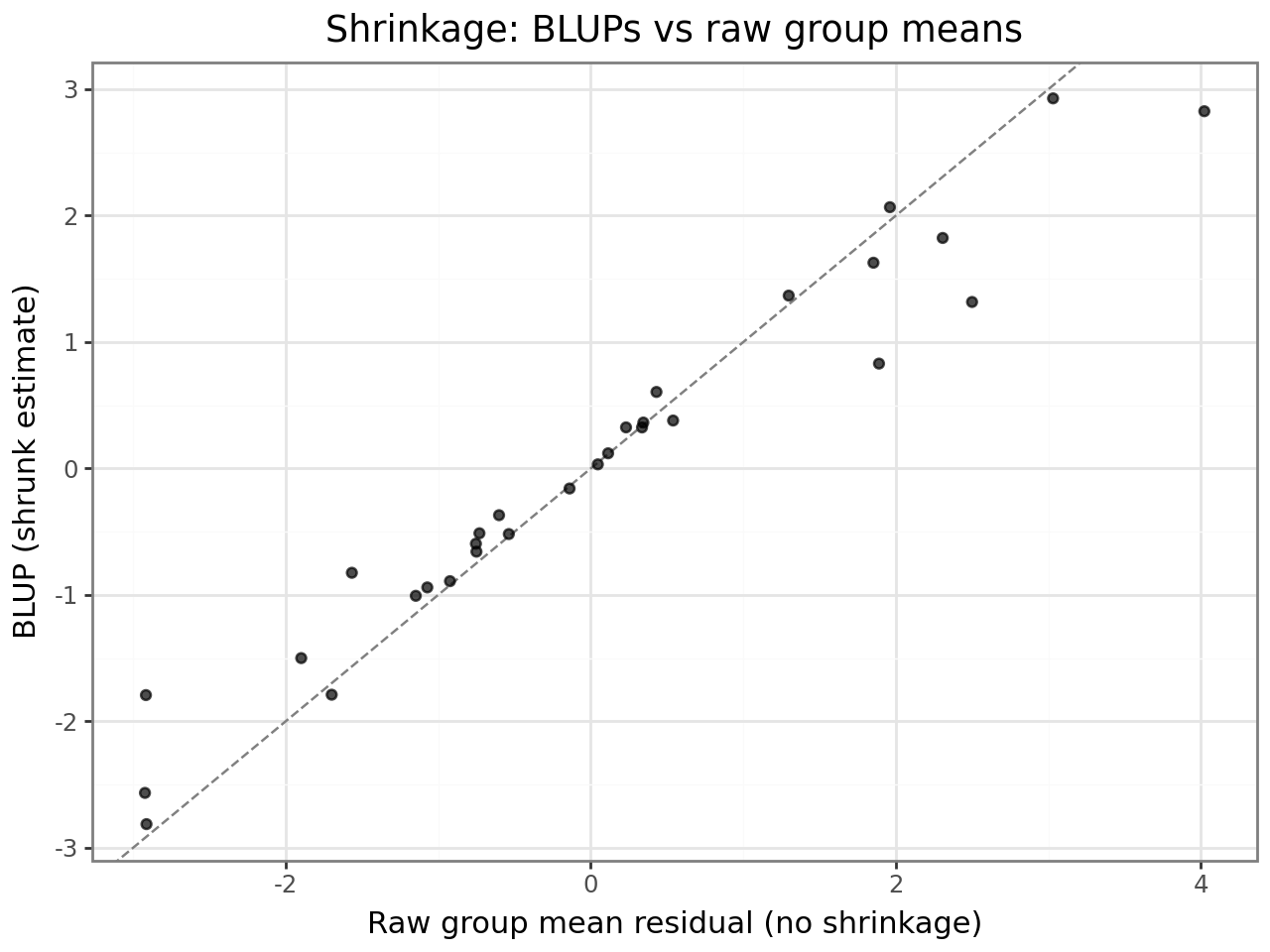
Shrinkage

BLUPs are shrunk toward zero relative to the group’s raw deviation. Groups with fewer observations or groups whose variance component is small are shrunk more. This is intentional: a student with only one observation should not be assigned an extreme intercept — the BLUP borrows strength from the population distribution.

The plot below makes shrinkage visible: each point is one student. Points above the diagonal are shrunk toward zero; the further from the line, the stronger the shrinkage.

from plotnine import ggplot, aes, geom_point, geom_abline, labs, theme_bw

raw = df.assign(resid=result.resid).groupby("student_id")["resid"].mean()

shrinkage_df = pd.DataFrame({
    "raw_mean_resid": raw,
    "blup":           student_blups.reindex(raw.index),
}).reset_index()

(
    ggplot(shrinkage_df, aes(x="raw_mean_resid", y="blup"))
    + geom_abline(slope=1, intercept=0, linetype="dashed", color="grey")
    + geom_point(alpha=0.7)
    + labs(
        x="Raw group mean residual (no shrinkage)",
        y="BLUP (shrunk estimate)",
        title="Shrinkage: BLUPs vs raw group means",
    )
    + theme_bw()
)

BLUPs vs fixed group dummies

BLUPs are not the same as including a fixed dummy variable for each group. Dummies use only the data from that group; BLUPs partially pool across groups. For groups with very many observations, BLUPs converge to the dummy-variable estimate. For small or sparse groups, BLUPs are much more stable.

---

Predictions

result.predict() returns fitted values, optionally including random effects.

	Conditional (include_re=True)	Marginal (include_re=False)
Includes BLUPs	Yes	No
Use case	In-sample fit, known groups	New groups, population-level
Unseen group levels	BLUP = 0 (shrinks to mean)	Identical to marginal

Conditional predictions are appropriate when you know which group an observation belongs to and want the best estimate for that specific group. They are used to compute residuals (result.resid = observed − conditional prediction).

Marginal predictions give the expected outcome for a hypothetical average group — useful for reporting population-level effects or when the new data includes groups not seen during training.

# Conditional predictions (uses BLUPs, default)
y_conditional = result.predict()

# Marginal predictions (fixed effects only)
y_marginal = result.predict(include_re=False)

print(f"Conditional predictions — mean: {y_conditional.mean():.2f}, std: {y_conditional.std():.2f}")
print(f"Marginal predictions    — mean: {y_marginal.mean():.2f}, std: {y_marginal.std():.2f}")

Conditional predictions — mean: 59.67, std: 1.43
Marginal predictions    — mean: 59.67, std: 1.43

Predicting on new data

Unseen group levels automatically receive a BLUP of zero — the population mean for that factor. This is the correct Bayesian-optimal behaviour under the model’s assumptions.

df_new = pd.DataFrame({
    "hours_studied": [5.0, 8.0, 5.0],
    "prior_gpa":     [3.2, 3.8, 3.2],
    "student_id":    ["s1", "s2", "s_new"],   # s_new is unseen → BLUP = 0
    "school_id":     ["sch1", "sch1", "sch1"],
})

preds = result.predict(newdata=df_new)

df_new.assign(predicted_score=preds.round(2))

	hours_studied	prior_gpa	student_id	school_id	predicted_score
0	5.0	3.2	s1	sch1	60.90
1	8.0	3.8	s2	sch1	58.98
2	5.0	3.2	s_new	sch1	59.58

---

Bootstrap standard error

For scalar statistics of the outcome (currently: median), bootstrap_se() computes a cluster-bootstrap standard error that respects the grouping structure.

Ordinary bootstrap resamples individual observations, which underestimates the SE when group variance is substantial. Cluster bootstrap resamples group levels with replacement, then includes all observations from the sampled groups — preserving within-group correlation.

Use resample_level="observation" only if you have verified that the ICC is negligible.

se_cluster     = result.bootstrap_se(statistic="median", n_bootstrap=500, resample_level="group",       seed=42)
se_observation = result.bootstrap_se(statistic="median", n_bootstrap=500, resample_level="observation", seed=42)

print(f"Median: {np.median(df['score']):.2f}")
print(f"Cluster-bootstrap SE:     {se_cluster:.4f}")
print(f"Observation-bootstrap SE: {se_observation:.4f}  (underestimates when ICC > 0)")

Median: 59.30
Cluster-bootstrap SE:     0.8252
Observation-bootstrap SE: 0.5958  (underestimates when ICC > 0)

---

Quick reference

Attribute	Type	What it tells you
fe_params	pd.Series	Fixed-effect coefficient estimates
fe_bse	pd.Series	Standard errors of fixed effects
fe_pvalues	pd.Series	Two-sided p-values (z-test)
fe_conf_int	pd.DataFrame	95% confidence intervals
fe_cov	np.ndarray	Fixed-effect covariance matrix
variance_components	dict	Between-group variance per factor
scale	float	Within-group (residual) variance σ²
random_effects	dict	BLUPs per grouping factor
fittedvalues	np.ndarray	Conditional fitted values
resid	np.ndarray	Conditional residuals
aic	float	Akaike Information Criterion
bic	float	Bayesian Information Criterion
llf	float	Log-likelihood at optimum
converged	bool	Whether the optimiser converged
nobs	int	Number of observations
ngroups	dict	Number of levels per grouping factor

---

Where to go next

• Diagnostics guide — residuals, leverage, Cook’s D, influence plots

• API: CrossedLMEResult — full attribute and method reference

• API: Prediction — predict() parameter details

• Concepts — background on REML, BLUPs, and variance components