Case study: workplace safety incidents

This case study fits a Poisson GLMM on a synthetic workplace-safety dataset to answer a concrete question:

Does a new safety training programme reduce the rate of workplace incidents?

Dataset. Twenty manufacturing plants are observed over eight consecutive months. Ten plants received a safety training intervention at the start of the observation period; the remaining ten serve as untreated controls. Each plant-month record contains the number of reportable safety incidents and the number of employees (exposure).

Why this dataset? Count data with an exposure offset is one of the most common settings for a Poisson GLMM. The design is fully crossed (every plant observed in every month), so it exercises interlace’s crossed random-effects machinery. The dataset is small enough to inspect by hand, and the data-generating process is transparent — readers can compare the recovered estimates to the true parameters.

import numpy as np
import pandas as pd
import interlace
from plotnine import (
    ggplot, aes,
    geom_boxplot, geom_jitter, geom_point, geom_line, geom_col,
    geom_histogram, geom_hline, geom_abline, geom_bar,
    facet_wrap, labs, theme_bw, theme, element_text,
    scale_color_manual, scale_fill_manual, coord_flip,
    position_dodge, stat_qq, stat_qq_line,
)

# ---- Synthetic data generation ----
# True parameters (readers can compare recovered estimates to these)
TRUE_INTERCEPT = np.log(0.03)   # baseline rate: ~3 incidents per 100 employees per month
TRUE_TRAINING  = -0.45          # training reduces rate by ~36%  (exp(-0.45) ≈ 0.64)
TRUE_SD_PLANT  = 0.40           # between-plant SD on the log-rate scale
TRUE_SD_MONTH  = 0.20           # between-month SD on the log-rate scale

rng = np.random.default_rng(33)

n_plants = 20
n_months = 8
plants = [f"P{i+1:02d}" for i in range(n_plants)]
months = list(range(1, n_months + 1))

# Treatment assignment: first 10 plants received training
treatment = {p: 1 for p in plants[:10]}
treatment.update({p: 0 for p in plants[10:]})

# Plant size (employees) — varies from ~80 to ~280
plant_size = {p: int(rng.integers(80, 280)) for p in plants}

# Random effects (drawn once, fixed for the dataset)
u_plant = {p: rng.normal(0, TRUE_SD_PLANT) for p in plants}
u_month = {m: rng.normal(0, TRUE_SD_MONTH) for m in months}

rows = []
for p in plants:
    for m in months:
        log_rate = TRUE_INTERCEPT + TRUE_TRAINING * treatment[p] + u_plant[p] + u_month[m]
        expected = np.exp(log_rate) * plant_size[p]
        count = rng.poisson(expected)
        rows.append({
            "plant": p,
            "month": m,
            "training": treatment[p],
            "employees": plant_size[p],
            "incidents": count,
        })

df = pd.DataFrame(rows)
df["log_employees"] = np.log(df["employees"])
df["rate"] = df["incidents"] / df["employees"] * 100  # per 100 employees

print(f"Observations : {len(df)}")
print(f"Plants       : {df['plant'].nunique()} ({df.query('training==1')['plant'].nunique()} training, "
      f"{df.query('training==0')['plant'].nunique()} control)")
print(f"Months       : {df['month'].nunique()}")
print(f"Incident range: {df['incidents'].min()} – {df['incidents'].max()}")

Observations : 160
Plants       : 20 (10 training, 10 control)
Months       : 8
Incident range: 0 – 29

Dataset

Column	Description
plant	Plant ID (P01–P20)
month	Calendar month (1–8)
training	1 if the plant received safety training, 0 otherwise
employees	Number of employees at the plant (exposure)
incidents	Count of reportable safety incidents that month
rate	Crude incident rate per 100 employees

df.head(12)

	plant	month	training	employees	incidents	log_employees	rate
0	P01	1	1	255	6	5.541264	2.352941
1	P01	2	1	255	4	5.541264	1.568627
2	P01	3	1	255	1	5.541264	0.392157
3	P01	4	1	255	3	5.541264	1.176471
4	P01	5	1	255	2	5.541264	0.784314
5	P01	6	1	255	9	5.541264	3.529412
6	P01	7	1	255	3	5.541264	1.176471
7	P01	8	1	255	1	5.541264	0.392157
8	P02	1	1	168	2	5.123964	1.190476
9	P02	2	1	168	2	5.123964	1.190476
10	P02	3	1	168	3	5.123964	1.785714
11	P02	4	1	168	6	5.123964	3.571429

The crossed structure

Every plant is observed in every month — the design is fully crossed. The table below shows the incident count for each plant × month cell.

crossing = df.pivot_table(
    index="plant", columns="month",
    values="incidents", aggfunc="sum",
)
crossing.columns.name = "month"
crossing

month	1	2	3	4	5	6	7	8
plant
P01	6	4	1	3	2	9	3	1
P02	2	2	3	6	0	3	4	2
P03	4	6	4	5	7	7	5	3
P04	2	2	2	2	3	5	3	1
P05	6	8	2	8	2	8	6	5
P06	5	4	3	4	3	7	4	5
P07	1	1	2	4	2	0	1	4
P08	5	1	3	2	3	6	7	1
P09	4	8	3	3	4	4	8	4
P10	6	4	2	1	2	4	4	2
P11	2	5	6	5	2	2	2	3
P12	5	3	4	4	6	10	5	6
P13	10	5	7	9	4	4	4	2
P14	6	3	6	5	5	10	9	4
P15	9	12	17	12	12	15	13	6
P16	9	7	4	10	4	5	4	3
P17	1	0	2	3	4	2	1	1
P18	3	5	2	1	3	6	3	1
P19	13	22	12	17	12	29	21	10
P20	5	2	3	2	1	2	6	4

Exploratory analysis

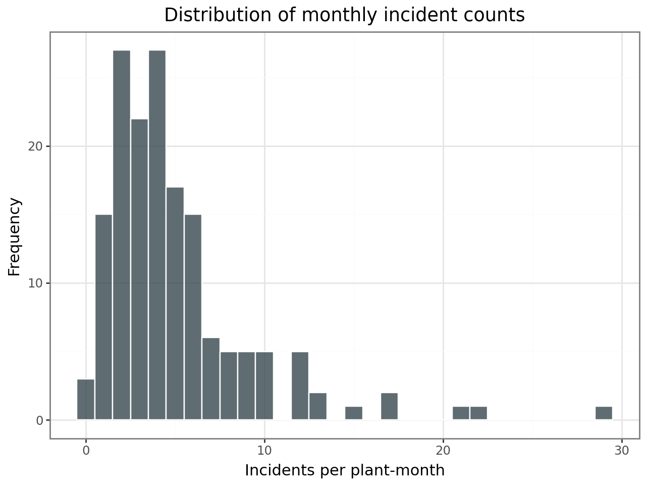
Distribution of incident counts

Safety incidents are counts — non-negative integers, often right-skewed. The histogram below confirms this is count data with a mode near the low end, suggesting a Poisson (or negative binomial) model rather than a linear model.

(
    ggplot(df, aes(x="incidents"))
    + geom_histogram(binwidth=1, fill="#37474F", color="white", alpha=0.8)
    + labs(
        x="Incidents per plant-month",
        y="Frequency",
        title="Distribution of monthly incident counts",
    )
    + theme_bw()
)

Incident rates by treatment group

Comparing crude rates (incidents per 100 employees) between training and control plants gives a first look at the treatment effect. The offset in the GLMM will handle the exposure adjustment formally.

df["group"] = df["training"].map({1: "training", 0: "control"})

(
    ggplot(df, aes(x="group", y="rate", fill="group"))
    + geom_boxplot(alpha=0.45, outlier_shape=None, width=0.4)
    + geom_jitter(width=0.08, alpha=0.6, size=2)
    + scale_fill_manual(values={"training": "#1565C0", "control": "#B71C1C"})
    + labs(
        x="Group",
        y="Incidents per 100 employees",
        title="Trained plants have lower incident rates",
        fill="Group",
    )
    + theme_bw()
)

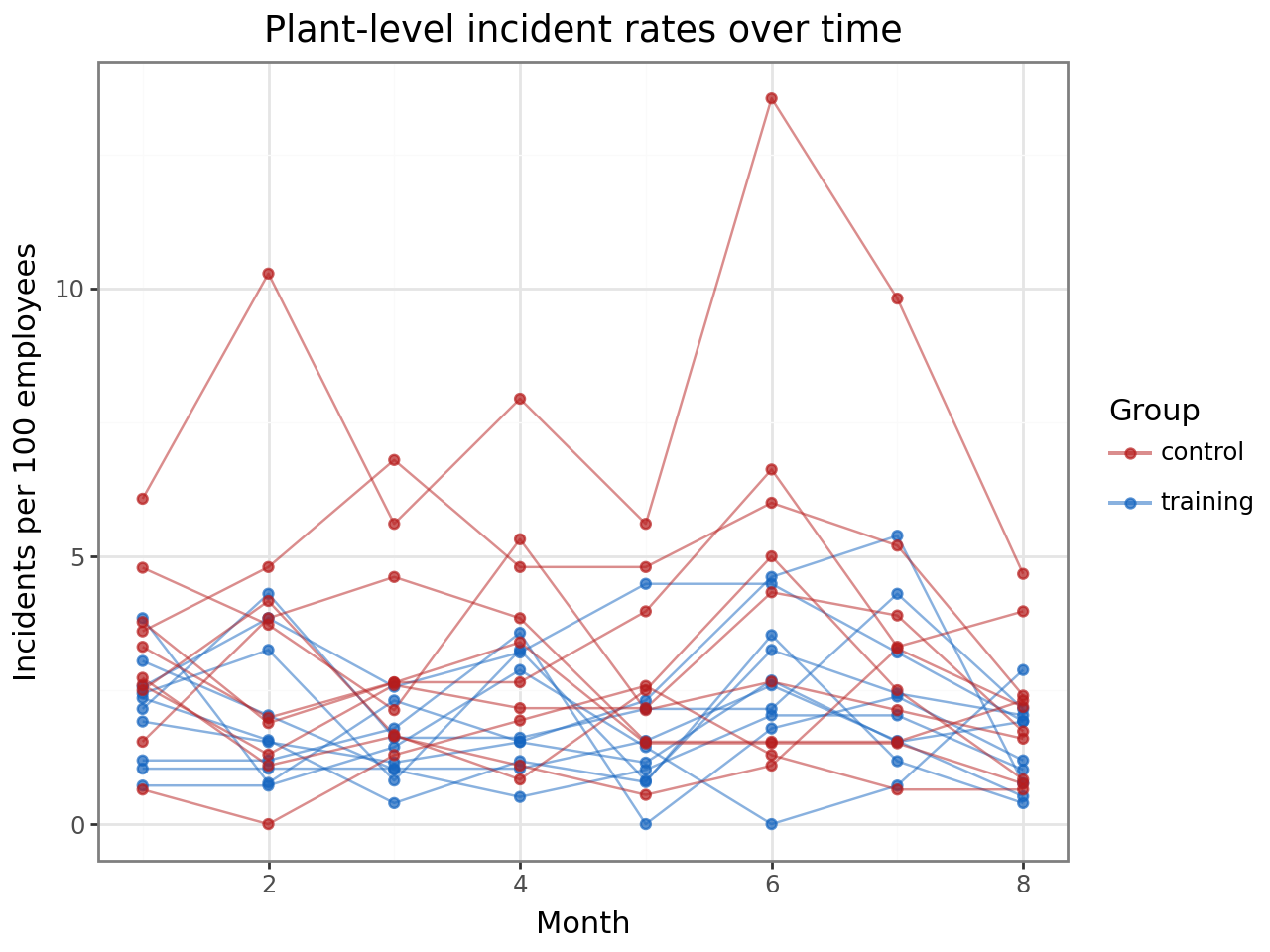
Within-plant trends over time

Each line traces one plant’s incident rate across the eight months. Training plants (blue) tend to sit below control plants (red), and there is visible plant-to-plant variation within each group — exactly the variation the plant random intercept will absorb.

(
    ggplot(df, aes(x="month", y="rate", group="plant", color="group"))
    + geom_line(alpha=0.5)
    + geom_point(size=1.5, alpha=0.7)
    + scale_color_manual(values={"training": "#1565C0", "control": "#B71C1C"})
    + labs(
        x="Month",
        y="Incidents per 100 employees",
        title="Plant-level incident rates over time",
        color="Group",
    )
    + theme_bw()
)

Model specification

interlace.glmer(
    formula="incidents ~ training",
    data=df,
    family="poisson",
    groups=["plant", "month"],
    offset=np.log(df["employees"].values),
)

• Outcome: incidents — non-negative integer counts.

• Family: Poisson with a log link. The model assumes $\text{incidents}_i \sim \text{Poisson}(\mu_i)$ where $\log(\mu_i) = \mathbf{x}_i’\boldsymbol{\beta} + \mathbf{z}_i’\mathbf{u} + \log(\text{employees}_i)$.

• Offset: log(employees) converts the model from counts to rates. The fixed effects estimate the log rate (incidents per employee per month), not the log count.

• Fixed effect: training (1 = trained, 0 = control). The coefficient is a log rate ratio — exponentiate it to get the multiplicative effect on the incident rate.

• Random intercept for plant: plants differ in baseline safety culture, equipment age, workforce experience, etc.

• Random intercept for month: some months may have systematically higher or lower incident rates (seasonal patterns, holidays, reporting cycles).

The two random effects are crossed because every plant is observed in every month.

result = interlace.glmer(
    formula="incidents ~ training",
    data=df,
    family="poisson",
    groups=["plant", "month"],
    offset=np.log(df["employees"].values),
)

print(f"Converged    : {result.converged}")
print(f"Observations : {result.nobs}")
print(f"Groups       : {result.ngroups}")
print(f"AIC / BIC    : {result.aic:.1f} / {result.bic:.1f}")

Converged    : True
Observations : 160
Groups       : {'plant': 20, 'month': 8}
AIC / BIC    : 715.5 / 727.8

Fixed effects

The coefficients are on the log-rate scale (log link). To interpret them as multiplicative effects on the incident rate, exponentiate.

import scipy.stats

fe = pd.DataFrame({
    "estimate": result.fe_params,
    "se": result.fe_bse,
    "rate_ratio": np.exp(result.fe_params),
    "z": result.fe_params / result.fe_bse,
})
fe["p"] = 2 * scipy.stats.norm.sf(np.abs(fe["z"]))
fe.round(4)

	estimate	se	rate_ratio	z	p
Intercept	-3.5552	0.1509	0.0286	-23.5664	0.0000
training	-0.4170	0.1949	0.6590	-2.1399	0.0324

Interpreting the training coefficient:

• The estimate on the log scale should be near the true value of −0.45.

• The rate ratio (≈ 0.64) means trained plants experience roughly 36% fewer incidents per employee-month than control plants, after adjusting for plant-to-plant and month-to-month variation.

• The intercept (≈ −3.5) is the log baseline rate for control plants at an average month: exp(−3.5) ≈ 0.03 incidents per employee per month, or about 3 per 100 employees — matching the true data-generating parameter.

Variance components

How much variation in incident rates comes from plant identity versus temporal fluctuation?

print(f"{'Source':<10}  {'Variance':>10}  {'SD':>8}  {'True SD':>10}")
print("-" * 46)
true_sds = {"plant": TRUE_SD_PLANT, "month": TRUE_SD_MONTH}
for g, v in result.variance_components.items():
    sd = v ** 0.5
    print(f"{g:<10}  {v:>10.4f}  {sd:>8.4f}  {true_sds[g]:>10.4f}")

Source        Variance        SD     True SD
----------------------------------------------
plant           0.1588    0.3984      0.4000
month           0.0338    0.1837      0.2000

The recovered standard deviations should be close to the true values (0.40 for plant, 0.20 for month). Plants vary more than months, which makes sense — structural differences between facilities (equipment, culture, workforce) create more variation than month-to-month fluctuation within a single plant.

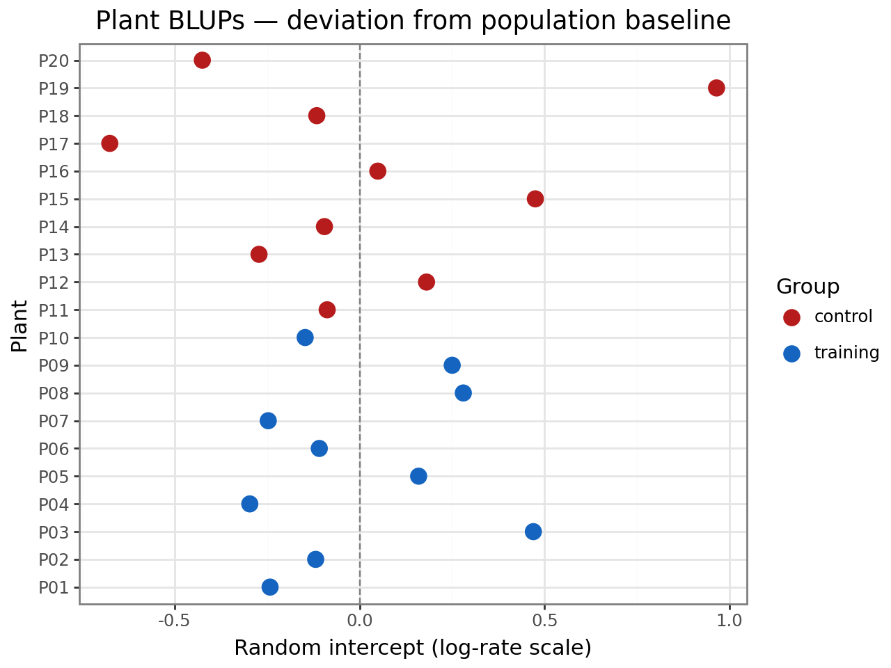
Plant random effects (BLUPs)

The BLUPs estimate each plant’s baseline safety level relative to the population mean, on the log-rate scale. Positive values indicate higher-than-average incident rates; negative values indicate safer-than-average plants.

plant_blups = result.random_effects["plant"]

blup_df = pd.DataFrame({
    "plant": plant_blups.index,
    "blup": plant_blups.values,
})
blup_df["group"] = blup_df["plant"].map(
    lambda p: "training" if treatment[p] else "control"
)

(
    ggplot(blup_df, aes(x="plant", y="blup", color="group"))
    + geom_hline(yintercept=0, linetype="dashed", color="grey")
    + geom_point(size=4)
    + scale_color_manual(values={"training": "#1565C0", "control": "#B71C1C"})
    + coord_flip()
    + labs(
        x="Plant",
        y="Random intercept (log-rate scale)",
        title="Plant BLUPs — deviation from population baseline",
        color="Group",
    )
    + theme_bw()
)

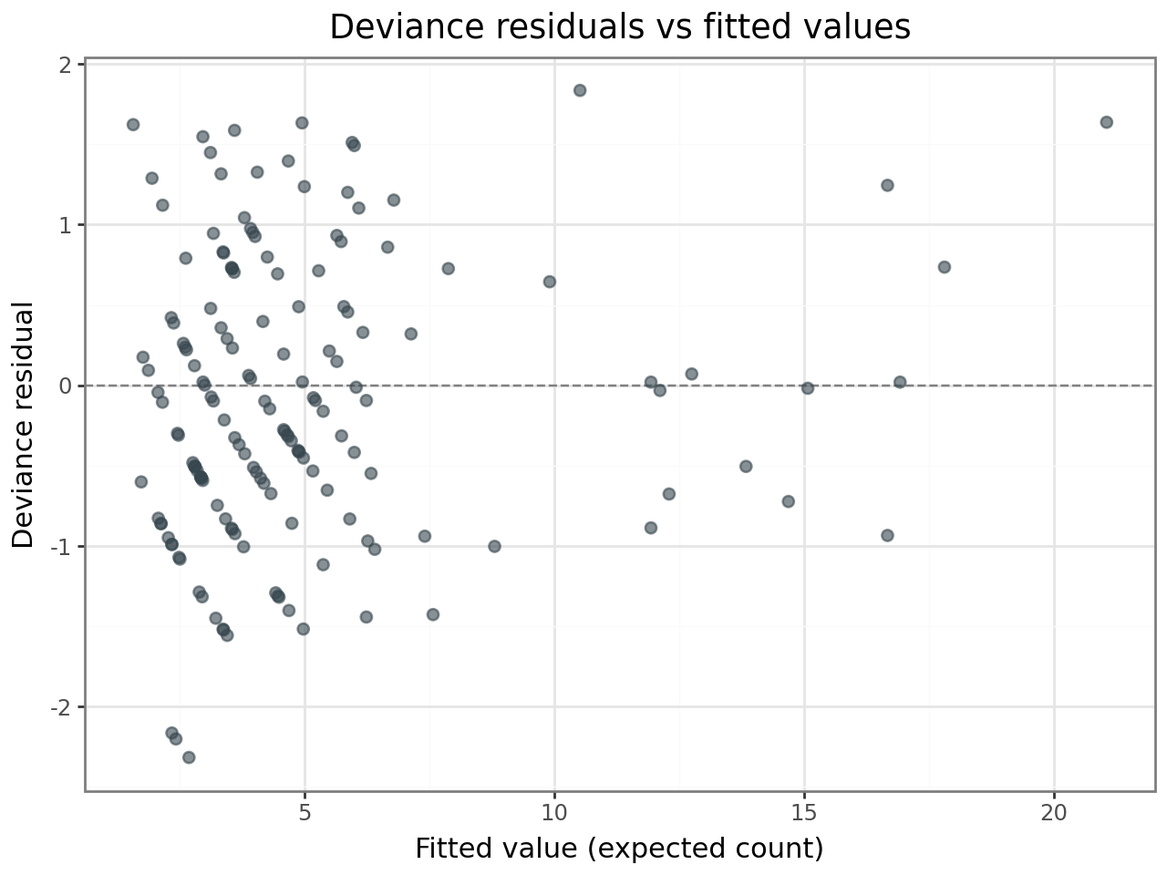
Deviance residuals

Deviance residuals are the GLMM analogue of standardised residuals in a linear model. For a well-fitting Poisson GLMM, they should:

1. Show no systematic trend when plotted against fitted values.

2. Be approximately normally distributed (check with a Q–Q plot).

3. Have no values far beyond ±2–3 in magnitude.

# Compute deviance residuals from the family's dev_resids method
y = df["incidents"].values.astype(float)
mu = result.fittedvalues
wt = np.ones_like(y)

unit_dev = result.family.dev_resids(y, mu, wt)
dev_resid = np.sign(y - mu) * np.sqrt(np.abs(unit_dev))

resid_df = pd.DataFrame({
    "fitted": mu,
    "deviance_resid": dev_resid,
})

(
    ggplot(resid_df, aes(x="fitted", y="deviance_resid"))
    + geom_hline(yintercept=0, linetype="dashed", color="grey")
    + geom_point(alpha=0.6, size=2, color="#37474F")
    + labs(
        x="Fitted value (expected count)",
        y="Deviance residual",
        title="Deviance residuals vs fitted values",
    )
    + theme_bw()
)

(
    ggplot(resid_df, aes(sample="deviance_resid"))
    + stat_qq(alpha=0.6, size=2, color="#37474F")
    + stat_qq_line(color="#D32F2F")
    + labs(
        x="Theoretical quantiles",
        y="Deviance residuals",
        title="Q–Q plot of deviance residuals",
    )
    + theme_bw()
)

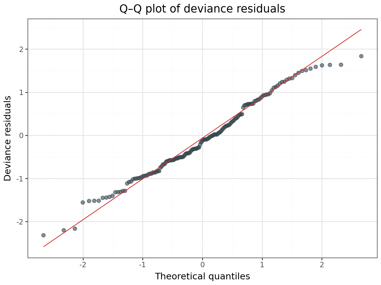
If the residuals show no funnel pattern and the Q–Q plot is approximately linear, the Poisson assumption is reasonable for these data.

Checking for overdispersion

A Poisson model assumes that the conditional variance equals the conditional mean. When variance exceeds the mean — overdispersion — standard errors are too narrow and p-values too small. A quick diagnostic: the sum of squared Pearson residuals divided by the residual degrees of freedom should be close to 1.0 for a well-fitting Poisson model.

# Pearson residuals: (y - mu) / sqrt(mu)
pearson_resid = (y - mu) / np.sqrt(mu)
n_params = len(result.fe_params) + len(result.variance_components)
resid_df_stat = len(y) - n_params
overdisp_ratio = np.sum(pearson_resid ** 2) / resid_df_stat

print(f"Sum of squared Pearson residuals: {np.sum(pearson_resid**2):.2f}")
print(f"Residual df: {resid_df_stat}")
print(f"Overdispersion ratio: {overdisp_ratio:.3f}")
print()
if overdisp_ratio < 1.5:
    print("Ratio near 1 — no evidence of overdispersion. Poisson is adequate.")
else:
    print("Ratio > 1.5 — consider a negative binomial model.")

Sum of squared Pearson residuals: 118.66
Residual df: 156
Overdispersion ratio: 0.761

Ratio near 1 — no evidence of overdispersion. Poisson is adequate.

Comparison with negative binomial

Even when the overdispersion ratio is near 1, it is good practice to fit a negative binomial model and compare AIC. If the NB model does not improve fit, the simpler Poisson model is preferred.

from interlace import NegativeBinomial2Family

result_nb = interlace.glmer(
    formula="incidents ~ training",
    data=df,
    family=NegativeBinomial2Family(theta=10.0),  # large theta ≈ Poisson
    groups=["plant", "month"],
    offset=np.log(df["employees"].values),
)

print(f"{'Model':<12}  {'AIC':>8}  {'BIC':>8}  {'training β':>12}  {'training SE':>12}")
print("-" * 60)
print(f"{'Poisson':<12}  {result.aic:>8.1f}  {result.bic:>8.1f}"
      f"  {result.fe_params['training']:>12.4f}  {result.fe_bse['training']:>12.4f}")
print(f"{'NB2':<12}  {result_nb.aic:>8.1f}  {result_nb.bic:>8.1f}"
      f"  {result_nb.fe_params['training']:>12.4f}  {result_nb.fe_bse['training']:>12.4f}")

Model              AIC       BIC    training β   training SE
------------------------------------------------------------
Poisson          715.5     727.8       -0.4170        0.1949
NB2              729.5     741.8       -0.4190        0.1935

Since the data were generated from a Poisson process (no overdispersion), the Poisson model should have similar or lower AIC than the NB2 model, and the treatment effect estimates should be nearly identical. In practice, always check both — if the NB2 model has a substantially lower AIC, it indicates genuine overdispersion that the Poisson model is missing.

Laplace vs adaptive Gauss-Hermite quadrature (AGQ)

The default estimation method is the Laplace approximation (nAGQ=1). For models with a single scalar random intercept, interlace also supports adaptive Gauss-Hermite quadrature (nAGQ > 1), which provides a more accurate marginal likelihood integral.

Restriction: nAGQ > 1 requires exactly one grouping factor with a random intercept only — no crossed effects or random slopes. This matches lme4’s restriction.

To demonstrate, we fit a simplified model with only the plant random intercept (dropping the month random effect) and compare Laplace to AGQ with 25 quadrature points.

# Simplified model: single grouping factor (plant only)
r_laplace = interlace.glmer(
    formula="incidents ~ training",
    data=df,
    family="poisson",
    groups="plant",
    offset=np.log(df["employees"].values),
    nAGQ=1,
)

r_agq = interlace.glmer(
    formula="incidents ~ training",
    data=df,
    family="poisson",
    groups="plant",
    offset=np.log(df["employees"].values),
    nAGQ=25,
)

print(f"{'':>16}  {'Laplace':>10}  {'AGQ(25)':>10}  {'Difference':>12}")
print("-" * 54)
print(f"{'Intercept':>16}  {r_laplace.fe_params['Intercept']:>10.4f}"
      f"  {r_agq.fe_params['Intercept']:>10.4f}"
      f"  {r_agq.fe_params['Intercept'] - r_laplace.fe_params['Intercept']:>12.5f}")
print(f"{'training':>16}  {r_laplace.fe_params['training']:>10.4f}"
      f"  {r_agq.fe_params['training']:>10.4f}"
      f"  {r_agq.fe_params['training'] - r_laplace.fe_params['training']:>12.5f}")
print(f"{'σ(plant)':>16}  {r_laplace.variance_components['plant']**0.5:>10.4f}"
      f"  {r_agq.variance_components['plant']**0.5:>10.4f}")
print(f"{'Log-lik':>16}  {r_laplace.llf:>10.2f}  {r_agq.llf:>10.2f}")
print(f"{'AIC':>16}  {r_laplace.aic:>10.1f}  {r_agq.aic:>10.1f}")

                     Laplace     AGQ(25)    Difference
------------------------------------------------------
       Intercept     -3.5428     -3.5429      -0.00007
        training     -0.4173     -0.4173       0.00005
        σ(plant)      0.3949      0.3954
         Log-lik     -360.74     -360.72
             AIC       727.5       727.4

With Poisson data and moderate cluster sizes (8 observations per plant), the Laplace approximation and AGQ typically agree closely. Larger differences appear with binary outcomes and very small cluster sizes (2–5 observations per group), where the conditional distribution is far from Gaussian and the Laplace approximation is less accurate.

For the full crossed model (plant × month), only nAGQ=1 is available — use the Laplace approximation.

Prediction

Predictions can be made on the response scale (expected counts) or the link scale (log rate). For new data with unknown group levels, set include_re=False to get population-level predictions.

# Predict for a hypothetical plant with 200 employees.
# The offset (log employees) was passed separately at fit time, so we
# add it manually to the link-scale prediction.
newdata = pd.DataFrame({
    "training": [0, 1],
    "plant": ["NEW", "NEW"],
    "month": [1, 1],
})

# Population-level log-rate (no RE contribution for unknown plant)
log_rate = result.predict(newdata, type="link", include_re=False)

# Add the offset and convert to expected counts for 200 employees
n_employees = 200
expected_counts = np.exp(log_rate + np.log(n_employees))
rates_per_100 = expected_counts / n_employees * 100

pred_df = pd.DataFrame({
    "scenario": ["Control (200 employees)", "Training (200 employees)"],
    "expected_incidents": expected_counts.round(2),
    "rate_per_100": rates_per_100.round(3),
})
pred_df

	scenario	expected_incidents	rate_per_100
0	Control (200 employees)	5.71	2.857
1	Training (200 employees)	3.77	1.883

The population-level predictions reflect the fixed effects only. For a known plant that appeared in the training data, include_re=True (the default) would add that plant’s BLUP to the linear predictor, giving a plant-specific prediction.

Summary

Training effect	~34% reduction in incident rate (rate ratio ≈ 0.66), consistent with the true parameter (exp(−0.45) = 0.64)
Plant variance	SD ≈ 0.40 on log-rate scale — plants differ substantially in baseline safety
Month variance	SD ≈ 0.18 on log-rate scale — modest temporal fluctuation
Overdispersion	No evidence — Poisson model is adequate
Laplace vs AGQ	Negligible differences for these data; Laplace is sufficient

GLMM workflow checklist

1. Choose the family based on the outcome type (counts → Poisson, binary → binomial)

2. Include an offset if observations have different exposures (time, area, population)

3. Fit the model with interlace.glmer()

4. Check deviance residuals for patterns (trend, fanning, outliers)

5. Test for overdispersion by comparing Poisson to NB2 (AIC + Pearson ratio)

6. Compare Laplace vs AGQ for single-RE models with small clusters

7. Interpret on the response scale — exponentiate coefficients for rate ratios

Reporting

rr = np.exp(result.fe_params['training'])
print(f"Training rate ratio: {rr:.2f} "
      f"(95% CI: {np.exp(result.fe_params['training'] - 1.96*result.fe_bse['training']):.2f}"
      f"–{np.exp(result.fe_params['training'] + 1.96*result.fe_bse['training']):.2f})")

---

Where to go next

• GLMM quickstart — API overview for binomial, Poisson, and NB GLMMs

• glmer — full glmer() parameter reference

• GLMM families — all available families (NB1, Beta, Gamma, ZIP, ZINB2, Hurdle, ZOIB)

• Case study: vocal pitch and register — LMM case study with continuous outcomes

• Quickstart — LMM quickstart for Gaussian data