Case Study: Teacher Effectiveness Ratings (CLMM)

This notebook demonstrates cumulative link mixed models (CLMM) using interlace.clmm() — the Python equivalent of R’s ordinal::clmm(). CLMMs are the right tool when your outcome is an ordered categorical variable (Likert scale, pain ratings, quality grades) and observations are clustered.

Scenario

We analyse synthetic teacher effectiveness ratings collected from students. The design:

Feature	Value
Teachers	20
Students per teacher	10
Total observations	200
Outcome	5-point rating (1 = poor … 5 = excellent)
Fixed effects	method (traditional / active), size (large / small)
Random effect	Teacher intercept
Design	Balanced 2×2, 5 teachers per cell

Both predictors vary at the teacher level (not within teacher), so the teacher random effect absorbs unmeasured instructor-level heterogeneity.

import numpy as np
import pandas as pd
import interlace
from scipy.special import expit
from plotnine import (
    ggplot, aes, geom_bar, geom_point, geom_errorbar, geom_line,
    facet_grid, facet_wrap, coord_flip, labs, theme_bw, theme,
    scale_fill_manual, scale_color_manual, scale_linetype_manual,
    element_text, element_blank, geom_hline, scale_y_continuous,
)

# True parameters
TRUE_THRESHOLDS = np.array([-2.0, -0.5, 0.8, 2.1])
TRUE_BETA_METHOD = 1.2   # active → higher ratings
TRUE_BETA_SIZE = -0.3    # small → slightly higher ratings
TRUE_SD_TEACHER = 0.8

rng = np.random.default_rng(42)

conditions = (
    [('traditional', 'large')] * 5 + [('traditional', 'small')] * 5 +
    [('active', 'large')] * 5 + [('active', 'small')] * 5
)
u_teacher = rng.normal(0, TRUE_SD_TEACHER, 20)

rows = []
for j in range(20):
    method, size = conditions[j]
    eta = (TRUE_BETA_METHOD * (method == 'active')
           + TRUE_BETA_SIZE * (size == 'small')
           + u_teacher[j])
    cum_probs = expit(TRUE_THRESHOLDS - eta)
    cat_probs = np.diff(np.concatenate([[0], cum_probs, [1]]))
    cat_probs = np.clip(cat_probs, 1e-10, None)
    cat_probs /= cat_probs.sum()
    ratings = rng.choice(np.arange(1, 6), size=10, p=cat_probs)
    for r in ratings:
        rows.append({'teacher': f'T{j+1:02d}', 'method': method,
                     'size': size, 'rating': int(r)})

df = pd.DataFrame(rows)
print(f"Shape: {df.shape}")
print("\nRating distribution:")
print(df['rating'].value_counts().sort_index())

Shape: (200, 4)

Rating distribution:
rating
1    23
2    52
3    43
4    42
5    40
Name: count, dtype: int64

df.head(8)

	teacher	method	size	rating
0	T01	traditional	large	4
1	T01	traditional	large	3
2	T01	traditional	large	5
3	T01	traditional	large	5
4	T01	traditional	large	4
5	T01	traditional	large	2
6	T01	traditional	large	3
7	T01	traditional	large	1

Exploratory Data Analysis

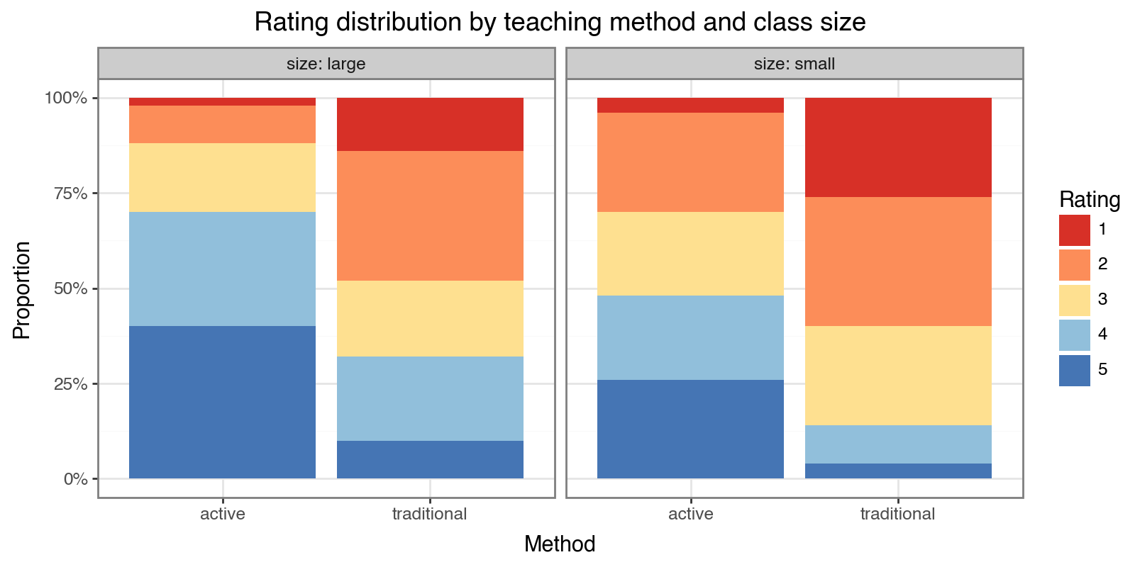
We expect active-method teachers to receive higher ratings, and small-class teachers to receive slightly higher ratings. The stacked proportional bar chart shows the rating distribution for each condition.

ORDINAL_PALETTE = ['#d73027', '#fc8d59', '#fee090', '#91bfdb', '#4575b4']

(
    ggplot(df, aes(x='method', fill='factor(rating)'))
    + geom_bar(position='fill')
    + facet_wrap('size', labeller='label_both')
    + scale_fill_manual(values=ORDINAL_PALETTE, name='Rating')
    + scale_y_continuous(labels=lambda l: [f"{v:.0%}" for v in l])
    + labs(
        title='Rating distribution by teaching method and class size',
        x='Method', y='Proportion',
    )
    + theme_bw()
    + theme(figure_size=(8, 4))
)

Model Specification

The cumulative link mixed model (proportional-odds formulation) is:

$$ \operatorname{logit}[P(Y_{ij} \leq k)] = \alpha_k - (\beta_1 \cdot \text{method}_j + \beta_2 \cdot \text{size}_j + u_j) $$

where $\alpha_1 < \alpha_2 < \alpha_3 < \alpha_4$ are the threshold parameters and $u_j \sim \mathcal{N}(0, \sigma^2)$ is the teacher random intercept.

The interlace.clmm() call mirrors statsmodels.MixedLM.from_formula(): a Wilkinson–Rogers formula for fixed effects, plus groups= for the clustering variable.

result = interlace.clmm(
    formula="rating ~ method + size",
    data=df,
    groups="teacher",
    link="logit",
)

print(f"Converged : {result.converged}")
print(f"N obs     : {result.nobs}")
print(f"AIC       : {result.aic:.2f}")
print(f"BIC       : {result.bic:.2f}")

Converged : True
N obs     : 200
AIC       : 595.22
BIC       : 618.30

thr = result.thresholds
thr_keys = list(thr.keys())
thr_values = np.array(list(thr.values()))
thr_df = pd.DataFrame({
    'threshold': thr_keys,
    'estimate': thr_values,
    'true': TRUE_THRESHOLDS,
    'abs_error': np.abs(thr_values - TRUE_THRESHOLDS),
})
print("Thresholds (logit scale — more negative = lower cumulative probability):")
thr_df.round(3)

Thresholds (logit scale — more negative = lower cumulative probability):

	threshold	estimate	true	abs_error
0	1|2	-3.730	-2.0	1.730
1	2|3	-1.927	-0.5	1.427
2	3|4	-0.829	0.8	1.629
3	4|5	0.409	2.1	1.691

ci = result.confint()          # DataFrame indexed by param name
# Keep only fixed-effect rows (exclude threshold rows)
fe_names = list(result.fe_params.index)
fe_ci = ci.loc[fe_names]

fe_table = pd.DataFrame({
    'estimate': result.fe_params,
    'SE':       result.fe_bse[fe_names],
    'OR':       np.exp(result.fe_params),
    'CI_lower': np.exp(fe_ci.iloc[:, 0]),
    'CI_upper': np.exp(fe_ci.iloc[:, 1]),
}, index=fe_names)

print("Fixed effects (OR = odds ratio for moving to a higher rating category):")
fe_table.round(3)

Fixed effects (OR = odds ratio for moving to a higher rating category):

	estimate	SE	OR	CI_lower	CI_upper
method[T.traditional]	-1.735	0.351	0.176	0.089	0.351
size[T.small]	-0.830	0.338	0.436	0.225	0.846

pred_grid = pd.DataFrame({
    'method':  ['traditional', 'traditional', 'active', 'active'],
    'size':    ['large',       'small',       'large',  'small'],
    'teacher': ['T_new'] * 4,
})

probs = result.predict(newdata=pred_grid, type="prob")

prob_df = pred_grid[['method', 'size']].copy()
for k in range(1, 6):
    prob_df[f'P({k})'] = probs[:, k - 1].round(3)

print("Predicted category probabilities for an average new teacher (u=0):")
prob_df

Predicted category probabilities for an average new teacher (u=0):

	method	size	P(1)	P(2)	P(3)	P(4)	P(5)
0	traditional	large	0.120	0.332	0.260	0.183	0.105
1	traditional	small	0.238	0.417	0.196	0.101	0.049
2	active	large	0.023	0.104	0.177	0.297	0.399
3	active	small	0.052	0.198	0.250	0.275	0.225

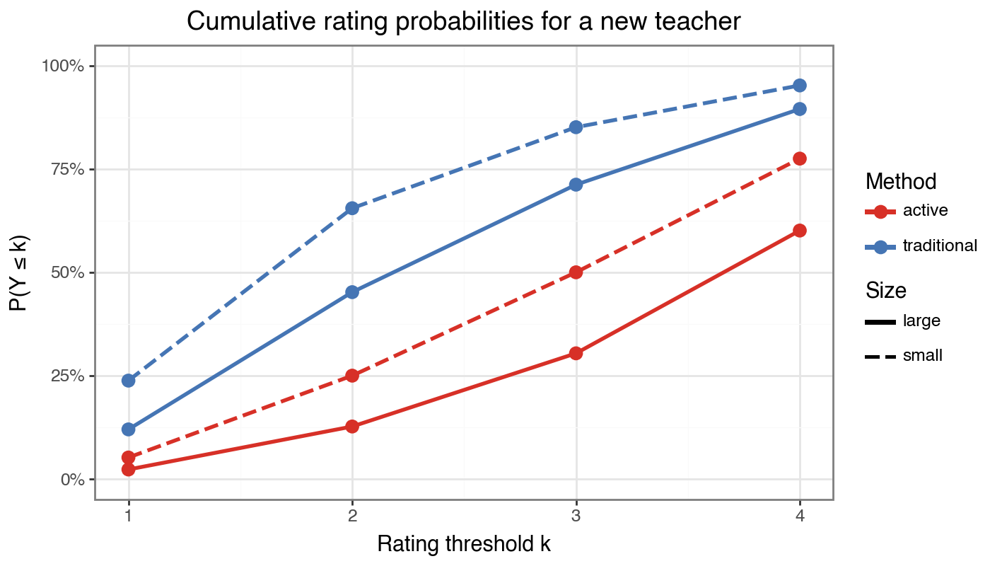
# Build cumulative probability curves P(Y <= k) for k=1..4
cum_rows = []
for _, row in prob_df.iterrows():
    cond = f"{row['method']}/{row['size']}"
    cump = 0.0
    for k in range(1, 5):
        cump += row[f'P({k})']
        cum_rows.append({'condition': cond, 'k': k, 'cum_prob': cump,
                         'method': row['method'], 'size': row['size']})

cum_df = pd.DataFrame(cum_rows)

(
    ggplot(cum_df, aes(x='k', y='cum_prob',
                       color='method', linetype='size', group='condition'))
    + geom_line(size=1.1)
    + geom_point(size=3)
    + scale_color_manual(values=['#d73027', '#4575b4'], name='Method')
    + scale_linetype_manual(values=['solid', 'dashed'], name='Size')
    + scale_y_continuous(limits=[0, 1],
                         labels=lambda l: [f"{v:.0%}" for v in l])
    + labs(
        title='Cumulative rating probabilities for a new teacher',
        x='Rating threshold k', y='P(Y \u2264 k)',
    )
    + theme_bw()
    + theme(figure_size=(7, 4))
)

# Teacher BLUPs with ±1.96 * teacher SD uncertainty bands
blups_series = result.random_effects['teacher']
teacher_sd = float(result.variance_components['teacher']) ** 0.5
half_width = 1.96 * teacher_sd

blup_df = pd.DataFrame({
    'teacher': blups_series.index,
    'blup': blups_series.values,
}).sort_values('blup').reset_index(drop=True)

# Attach method info for colouring
teacher_meta = df.drop_duplicates('teacher')[['teacher', 'method']]
blup_df = blup_df.merge(teacher_meta, on='teacher')
blup_df['teacher'] = pd.Categorical(blup_df['teacher'],
                                     categories=blup_df['teacher'].tolist(),
                                     ordered=True)

(
    ggplot(blup_df, aes(x='teacher', y='blup', color='method'))
    + geom_hline(yintercept=0, linetype='dashed', color='grey60')
    + geom_errorbar(
        aes(ymin='blup - ' + str(half_width),
            ymax='blup + ' + str(half_width)),
        width=0.4,
    )
    + geom_point(size=3)
    + coord_flip()
    + scale_color_manual(values=['#d73027', '#4575b4'], name='Method')
    + labs(
        title='Teacher BLUPs (sorted) with \u00b11.96\u00d7SD bands',
        x='Teacher', y='Random intercept (logit scale)',
    )
    + theme_bw()
    + theme(figure_size=(6, 7),
            axis_text_y=element_text(size=8))
)

---------------------------------------------------------------------------
KeyError                                  Traceback (most recent call last)
File ~/repos/gpg/interlace/.venv/lib/python3.14/site-packages/mizani/_colors/named_colors.py:20, in _color_lookup.__getitem__(self, key)
     19 try:
---> 20     return super().__getitem__(key)
     21 except KeyError as err:

KeyError: 'grey60'

The above exception was the direct cause of the following exception:

ValueError                                Traceback (most recent call last)
File ~/repos/gpg/interlace/.venv/lib/python3.14/site-packages/IPython/core/formatters.py:1036, in MimeBundleFormatter.__call__(self, obj, include, exclude)
   1033     method = get_real_method(obj, self.print_method)
   1035     if method is not None:
-> 1036         return method(include=include, exclude=exclude)
   1037     return None
   1038 else:

File ~/repos/gpg/interlace/.venv/lib/python3.14/site-packages/plotnine/ggplot.py:172, in ggplot._repr_mimebundle_(self, include, exclude)
    169     self.theme = self.theme.to_retina()
    171 buf = BytesIO()
--> 172 self.save(buf, "png" if format == "retina" else format, verbose=False)
    173 figure_size_px = self.theme._figure_size_px
    174 return get_mimebundle(buf.getvalue(), format, figure_size_px)

File ~/repos/gpg/interlace/.venv/lib/python3.14/site-packages/plotnine/ggplot.py:681, in ggplot.save(self, filename, format, path, width, height, units, dpi, limitsize, verbose, **kwargs)
    632 def save(
    633     self,
    634     filename: Optional[str | Path | BytesIO] = None,
   (...)    643     **kwargs: Any,
    644 ):
    645     """
    646     Save a ggplot object as an image file
    647 
   (...)    679         Additional arguments to pass to matplotlib `savefig()`.
    680     """
--> 681     sv = self.save_helper(
    682         filename=filename,
    683         format=format,
    684         path=path,
    685         width=width,
    686         height=height,
    687         units=units,
    688         dpi=dpi,
    689         limitsize=limitsize,
    690         verbose=verbose,
    691         **kwargs,
    692     )
    694     with plot_context(self).rc_context:
    695         sv.figure.savefig(**sv.kwargs)

File ~/repos/gpg/interlace/.venv/lib/python3.14/site-packages/plotnine/ggplot.py:629, in ggplot.save_helper(self, filename, format, path, width, height, units, dpi, limitsize, verbose, **kwargs)
    626 if dpi is not None:
    627     self.theme = self.theme + theme(dpi=dpi)
--> 629 figure = self.draw(show=False)
    630 return mpl_save_view(figure, fig_kwargs)

File ~/repos/gpg/interlace/.venv/lib/python3.14/site-packages/plotnine/ggplot.py:314, in ggplot.draw(self, show)
    311 self.theme.setup(self)
    313 # Drawing
--> 314 self._draw_layers()
    315 self._draw_panel_borders()
    316 self._draw_breaks_and_labels()

File ~/repos/gpg/interlace/.venv/lib/python3.14/site-packages/plotnine/ggplot.py:461, in ggplot._draw_layers(self)
    457 """
    458 Draw the main plot(s) onto the axes.
    459 """
    460 # Draw the geoms
--> 461 self.layers.draw(self.layout, self.coordinates)

File ~/repos/gpg/interlace/.venv/lib/python3.14/site-packages/plotnine/layer.py:481, in Layers.draw(self, layout, coord)
    479 def draw(self, layout: Layout, coord: coord):
    480     for l in self:
--> 481         l.draw(layout, coord)

File ~/repos/gpg/interlace/.venv/lib/python3.14/site-packages/plotnine/layer.py:377, in layer.draw(self, layout, coord)
    374 self.data = self.geom.handle_na(self.data)
    375 # At this point each layer must have the data
    376 # that is created by the plot build process
--> 377 self.geom.draw_layer(self.data, layout, coord)

File ~/repos/gpg/interlace/.venv/lib/python3.14/site-packages/plotnine/geoms/geom.py:326, in geom.draw_layer(self, data, layout, coord)
    324 panel_params = layout.panel_params[ploc]
    325 ax = layout.axs[ploc]
--> 326 self.draw_panel(pdata, panel_params, coord, ax)

File ~/repos/gpg/interlace/.venv/lib/python3.14/site-packages/plotnine/geoms/geom_hline.py:96, in geom_hline.draw_panel(self, data, panel_params, coord, ax)
     94 for _, gdata in data.groupby("group"):
     95     gdata.reset_index(inplace=True)
---> 96     geom_segment.draw_group(
     97         gdata, panel_params, coord, ax, self.params
     98     )

File ~/repos/gpg/interlace/.venv/lib/python3.14/site-packages/plotnine/geoms/geom_segment.py:73, in geom_segment.draw_group(data, panel_params, coord, ax, params)
     71 data = coord.transform(data, panel_params)
     72 linewidth = data["size"] * SIZE_FACTOR
---> 73 color = to_rgba(data["color"], data["alpha"])
     75 # start point -> end point, sequence of xy points
     76 # from which line segments are created
     77 x = interleave(data["x"], data["xend"])

File ~/repos/gpg/interlace/.venv/lib/python3.14/site-packages/mizani/_colors/utils.py:130, in to_rgba(colors, alpha)
    128     return [to_rgba(c, alpha) for c in colors]  # pyright: ignore[reportCallIssue,reportArgumentType]
    129 else:
--> 130     return [to_rgba(c, a) for c, a in zip(colors, alpha)]

File ~/repos/gpg/interlace/.venv/lib/python3.14/site-packages/mizani/_colors/utils.py:110, in to_rgba(colors, alpha)
    107     return "none"
    109 if isinstance(alpha, (float, int, np.floating, np.integer)):
--> 110     c = get_named_color(colors)
    111     if len(c) > 7:
    112         return c

File ~/repos/gpg/interlace/.venv/lib/python3.14/site-packages/mizani/_colors/named_colors.py:72, in get_named_color(name)
     70     return name
     71 else:
---> 72     return NAMED_COLORS[name.lower()]

File ~/repos/gpg/interlace/.venv/lib/python3.14/site-packages/mizani/_colors/named_colors.py:22, in _color_lookup.__getitem__(self, key)
     20     return super().__getitem__(key)
     21 except KeyError as err:
---> 22     raise ValueError(f"Unknown name '{key}' for a color.") from err

ValueError: Unknown name 'grey60' for a color.

<plotnine.ggplot.ggplot object at 0x1237bcbb0>

result_probit = interlace.clmm(
    formula="rating ~ method + size",
    data=df,
    groups="teacher",
    link="probit",
)

compare = pd.DataFrame({
    'logit_est':  result.fe_params.round(3).values,
    'logit_SE':   result.fe_bse[fe_names].round(3).values,
    'probit_est': result_probit.fe_params.round(3).values,
    'probit_SE':  result_probit.fe_bse[fe_names].round(3).values,
}, index=fe_names)

print("Logit vs probit link — fixed effects:")
print(compare.to_string())
print(f"\nLogit  AIC: {result.aic:.2f}  |  Probit AIC: {result_probit.aic:.2f}")
print("(Estimates on probit scale are ~0.59× logit — the π/√3 rescaling)")

Logit vs probit link — fixed effects:
                       logit_est  logit_SE  probit_est  probit_SE
method[T.traditional]     -1.735     0.351      -1.033      0.198
size[T.small]             -0.830     0.338      -0.480      0.193

Logit  AIC: 595.22  |  Probit AIC: 594.35
(Estimates on probit scale are ~0.59× logit — the π/√3 rescaling)

Summary

Workflow checklist for CLMMs with interlace:

• [ ] Confirm the outcome is genuinely ordered (not nominal).

• [ ] Identify the clustering variable and check group sizes.

• [ ] Call interlace.clmm(formula, data, groups, link="logit") and verify result.converged.

• [ ] Inspect thresholds for ordering ($\alpha_1 < \alpha_2 < \ldots$).

• [ ] Interpret fixed-effect odds ratios (logit link) or cumulative probability shifts.

• [ ] Use result.predict(newdata, type="prob") for marginal predictions at new group levels.

• [ ] Check the BLUP caterpillar plot — wide spread indicates substantial teacher heterogeneity.

• [ ] Compare logit vs probit AIC to confirm link choice.

Where to go next:

• CLMM quickstart — minimal working example and API reference

• clmm — full parameter and return-value documentation

• Case study: workplace safety incidents — count outcomes (Poisson/NB) with crossed random effects