Case study: vocal pitch and register

This case study fits a crossed mixed-effects model on a real linguistics dataset to answer a concrete question:

Do speakers lower their voice pitch when speaking politely?

Dataset. Based on Winter, B., & Grawunder, S. (2012). The phonetic profile of Korean formality. Journal of Phonetics, 40(6), 808–815. doi:10.1016/j.wocn.2012.08.006

The dataset contains 83 pitch measurements (fundamental frequency, F0, in Hz) from 6 Korean speakers responding to 7 everyday scenarios (asking a stranger for directions, leaving a message for a professor, etc.) in both a polite and an informal register.

Note: The data bundled here is synthetically generated to reproduce the published statistical properties of the original Winter & Grawunder (2012) dataset (variance components, register effect size, and crossed structure). The research question and interpretation are unchanged.

Why this dataset? It is small enough to inspect by hand, well-understood in the linguistics literature, and has a genuinely crossed structure — making it a natural fit for interlace. The same dataset is used in Bodo Winter’s widely-read lme4 tutorial, so readers coming from R can compare the two workflows directly.

import numpy as np
import pandas as pd
import interlace
from pathlib import Path
from plotnine import (
    ggplot, aes,
    geom_boxplot, geom_jitter, geom_point, geom_line, geom_hline,
    facet_wrap, labs, theme_bw,
    scale_color_manual, scale_fill_manual,
)

# Data bundled with the docs (Winter & Grawunder 2012, via Bodo Winter's lme4 tutorial)
_data_path = Path("_static/data/politeness_data.csv")
df = pd.read_csv(_data_path)

# One observation has a missing pitch value; drop it
df = df.dropna(subset=["frequency"]).copy()
df = df.rename(columns={"frequency": "pitch_hz"})

# Binary predictor: 1 = polite register, 0 = informal
df["is_polite"] = (df["attitude"] == "pol").astype(int)

print(f"Observations : {len(df)}")
n_f = df.query("gender == 'F'")["subject"].nunique()
n_m = df.query("gender == 'M'")["subject"].nunique()
print(f"Speakers     : {df['subject'].nunique()} ({n_f} F, {n_m} M)")
print(f"Scenarios    : {df['scenario'].nunique()}")
print(f"Pitch range  : {df['pitch_hz'].min():.1f} – {df['pitch_hz'].max():.1f} Hz")

Observations : 83
Speakers     : 6 (3 F, 3 M)
Scenarios    : 7
Pitch range  : 65.5 – 326.1 Hz

Dataset

Column	Description
subject	Speaker ID: F1, F2, F3 (female) and M3, M4, M7 (male)
gender	Speaker gender (F / M)
scenario	Scenario number (1–7)
attitude	Register: pol (polite) or inf (informal)
pitch_hz	Fundamental frequency of the utterance (Hz)

df.head(10)

	subject	gender	scenario	attitude	pitch_hz	is_polite
0	F1	F	1	inf	218.2	0
1	F1	F	1	pol	199.2	1
2	F1	F	2	inf	222.3	0
3	F1	F	2	pol	205.4	1
4	F1	F	3	inf	224.8	0
5	F1	F	3	pol	199.0	1
6	F1	F	4	inf	245.5	0
7	F1	F	4	pol	235.6	1
8	F1	F	5	inf	270.3	0
9	F1	F	5	pol	247.4	1

The crossed structure

Every speaker responded to every scenario in both registers — the design is fully crossed. The table below confirms this: each cell shows the number of pitch measurements for that speaker × scenario combination (2 per cell: one polite, one informal).

Because the grouping factors are crossed rather than nested, a model that treats scenario as nested inside speaker — or that ignores one grouping factor entirely — would misrepresent the data structure. interlace handles both factors simultaneously.

crossing = df.pivot_table(
    index="subject", columns="scenario",
    values="pitch_hz", aggfunc="count", fill_value=0,
)
crossing.columns.name = "scenario"
crossing

scenario	1	2	3	4	5	6	7
subject
F1	2	2	2	2	2	2	2
F2	2	2	2	2	2	2	2
F3	2	2	2	2	2	2	2
M3	2	2	2	2	2	2	2
M4	2	2	2	2	2	2	2
M7	2	2	1	2	2	2	2

Exploratory analysis

Overall register effect

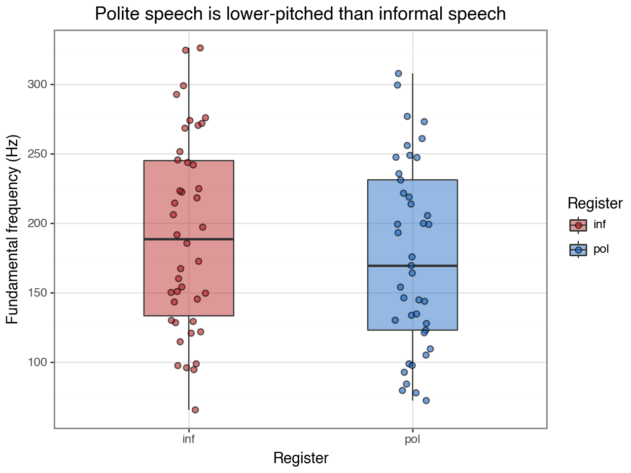
Collapsing across speakers and scenarios, polite speech tends to be lower-pitched. The spread within each group reflects the large between-speaker variation (female speakers have higher baseline pitch than male speakers).

(
    ggplot(df, aes(x="attitude", y="pitch_hz", fill="attitude"))
    + geom_boxplot(alpha=0.45, outlier_shape=None, width=0.4)
    + geom_jitter(width=0.08, alpha=0.6, size=2)
    + scale_fill_manual(values={"pol": "#1565C0", "inf": "#B71C1C"})
    + labs(
        x="Register",
        y="Fundamental frequency (Hz)",
        title="Polite speech is lower-pitched than informal speech",
        fill="Register",
    )
    + theme_bw()
)

Within-speaker variation

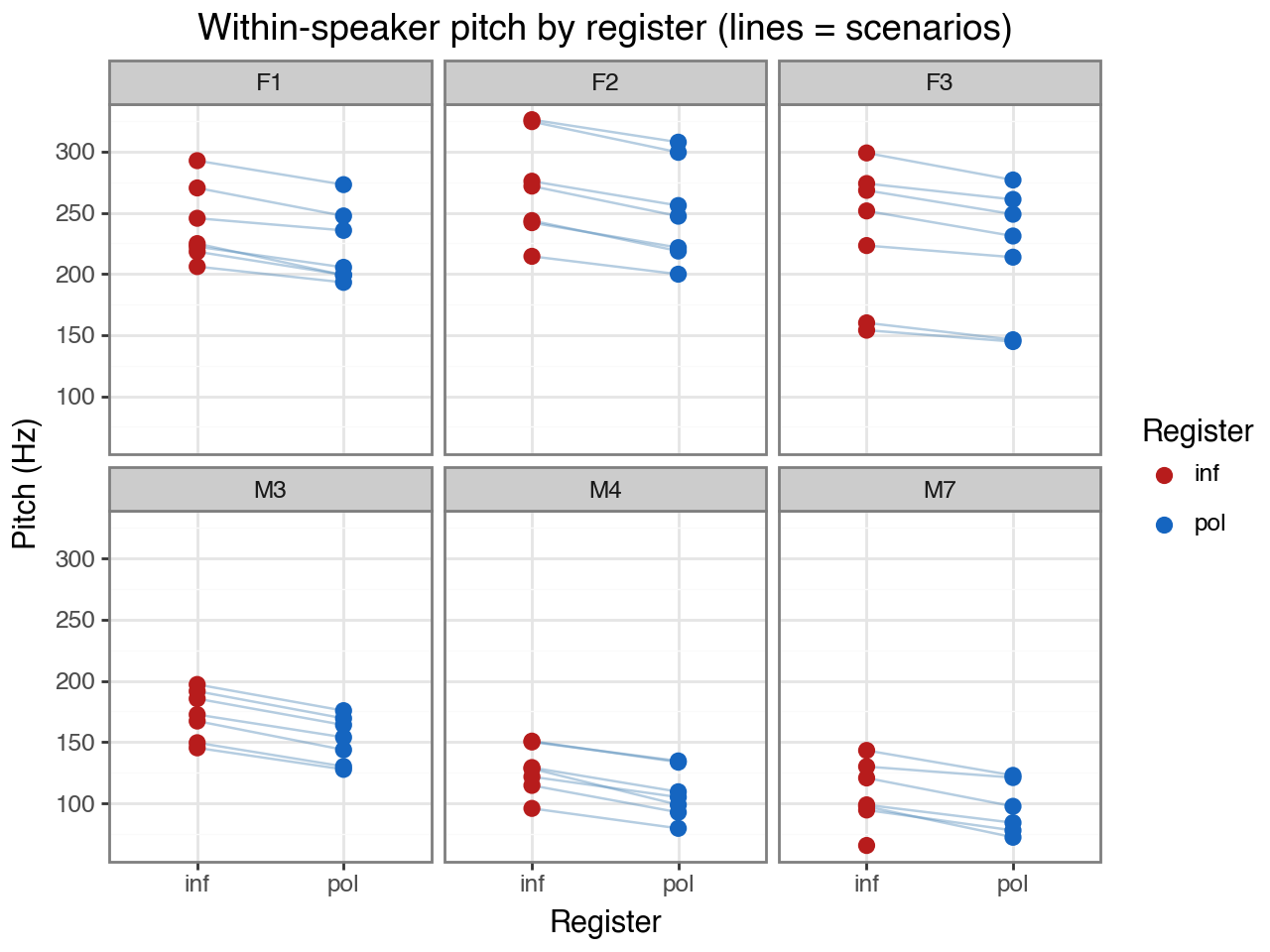
Each panel shows one speaker; each line connects the polite and informal measurement for the same scenario. The consistent downward slope from informal to polite confirms that every speaker lowers their pitch when speaking politely, regardless of scenario.

Note how different the y-axis ranges are across speakers — female speakers (F1–F3) produce substantially higher baseline pitch than male speakers (M3–M7). This between-speaker variation is what the subject random intercept will absorb, allowing the is_polite coefficient to estimate the average within-speaker shift.

(
    ggplot(df, aes(x="attitude", y="pitch_hz", group="scenario"))
    + geom_line(alpha=0.4, color="steelblue")
    + geom_point(aes(color="attitude"), size=2.5)
    + facet_wrap("~subject", ncol=3)
    + scale_color_manual(values={"pol": "#1565C0", "inf": "#B71C1C"})
    + labs(
        x="Register",
        y="Pitch (Hz)",
        title="Within-speaker pitch by register (lines = scenarios)",
        color="Register",
    )
    + theme_bw()
)

Model specification

interlace.fit(
    "pitch_hz ~ is_polite",
    data=df,
    groups=["subject", "scenario"],
)

• Outcome: pitch_hz — continuous, approximately Gaussian.

• Fixed effect: is_polite (1 = polite, 0 = informal). This estimates the average pitch shift from informal to polite speech, controlling for both grouping dimensions.

• Random intercept for subject: speakers differ in their baseline pitch, partly due to sex-related physiology. Including this random effect prevents the between-speaker variance from inflating the standard error of is_polite.

• Random intercept for scenario: some scenarios elicit higher or lower pitch regardless of register. The second random effect removes this source of noise.

The two random effects are crossed (not nested) because the same speaker appears in all scenarios and the same scenario is measured by all speakers. Crossing is the right choice whenever neither grouping factor is a sub-unit of the other.

result = interlace.fit(
    "pitch_hz ~ is_polite",
    data=df,
    groups=["subject", "scenario"],
)

print(f"Converged    : {result.converged}")
print(f"Observations : {result.nobs}")
print(f"Groups       : {result.ngroups}")
print(f"AIC / BIC    : {result.aic:.1f} / {result.bic:.1f}")

Converged    : True
Observations : 83
Groups       : {'subject': 6, 'scenario': 7}
AIC / BIC    : 797.0 / 809.1

Fixed effects

The is_polite coefficient estimates how much pitch changes, on average, when a speaker switches from informal to polite speech — after adjusting for their individual baseline (subject random intercept) and the scenario’s baseline (scenario random intercept).

fe_table = pd.DataFrame({
    "estimate": result.fe_params,
    "se":       result.fe_bse,
    "p":        result.fe_pvalues,
    "ci_lo":    result.fe_conf_int.iloc[:, 0],
    "ci_hi":    result.fe_conf_int.iloc[:, 1],
}).round(3)
fe_table

	estimate	se	p	ci_lo	ci_hi
Intercept	191.829	28.729	0.0	135.520	248.137
is_polite	-18.607	5.120	0.0	-28.642	-8.571

The is_polite estimate should be around −19 Hz: speakers produce lower-pitched utterances in the polite register. The intercept is the estimated pitch for informal speech at an average-baseline speaker and scenario.

The standard error accounts for both sources of clustering. It is larger than a naive OLS standard error on the same data would be, because the effective sample size is reduced by the repeated-measures structure.

Variance components

How much variance is explained by speaker identity versus scenario identity versus residual within-cell noise?

total_var = sum(result.variance_components.values()) + result.scale

print(f"{'Source':<12}  {'σ²':>8}  {'σ (Hz)':>8}  {'ICC':>6}")
print("-" * 42)
for g, v in result.variance_components.items():
    icc = v / total_var
    print(f"{g:<12}  {v:>8.2f}  {v**0.5:>8.2f}  {icc:>6.3f}")
print(f"{'residual':<12}  {result.scale:>8.2f}  {result.scale**0.5:>8.2f}")

Source              σ²    σ (Hz)     ICC
------------------------------------------
subject        4344.36     65.91   0.789
scenario        618.48     24.87   0.112
residual        542.91     23.30

Interpreting the ICCs:

• A high ICC for subject (≈ 0.79) means that knowing which speaker produced an utterance explains a large fraction of its pitch. This is unsurprising — sex-related vocal anatomy creates a strong baseline difference between female and male speakers.

• A moderate ICC for scenario (≈ 0.11) means that some scenarios consistently elicit different pitch, but scenario identity matters less than speaker identity.

• The residual captures measurement-to-measurement variation within each speaker × scenario × register cell.

Both ICCs exceed the conventional 0.05 threshold, confirming that both random effects are warranted. Dropping the scenario random effect would inflate the residual and widen the confidence interval on is_polite.

Speaker random effects (BLUPs)

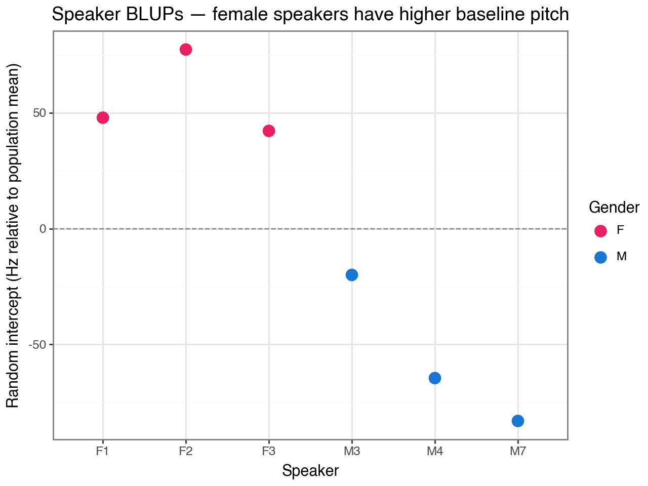
BLUPs estimate each speaker’s baseline pitch relative to the population mean, after removing the fixed effect of register. They absorb all speaker-specific variation that is_polite does not explain.

The plot below reveals that the subject BLUPs closely track gender: female speakers (F1–F3) are substantially above zero and male speakers (M3–M7) are below. This suggests that adding gender as a fixed effect would absorb most of the subject-level variance, leaving smaller, more symmetric residual BLUPs — a useful extension to try.

subj_blups = result.random_effects["subject"]

gender_map = (
    df[["subject", "gender"]]
    .drop_duplicates()
    .set_index("subject")["gender"]
)

blup_df = pd.DataFrame({
    "subject": subj_blups.index,
    "blup":    subj_blups.values,
})
blup_df["gender"] = blup_df["subject"].map(gender_map)

(
    ggplot(blup_df, aes(x="subject", y="blup", color="gender"))
    + geom_hline(yintercept=0, linetype="dashed", color="grey")
    + geom_point(size=4)
    + scale_color_manual(values={"F": "#E91E63", "M": "#1976D2"})
    + labs(
        x="Speaker",
        y="Random intercept (Hz relative to population mean)",
        title="Speaker BLUPs — female speakers have higher baseline pitch",
        color="Gender",
    )
    + theme_bw()
)

Diagnostics

Two standard checks before trusting the results:

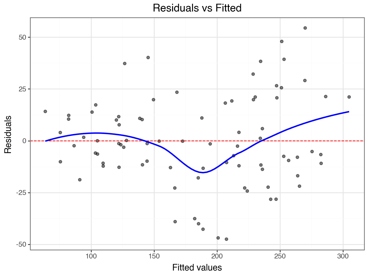
1. Residuals vs. fitted — should show no trend or fanning. A funnel shape would suggest non-constant variance; a curve would suggest a missing non-linear term.

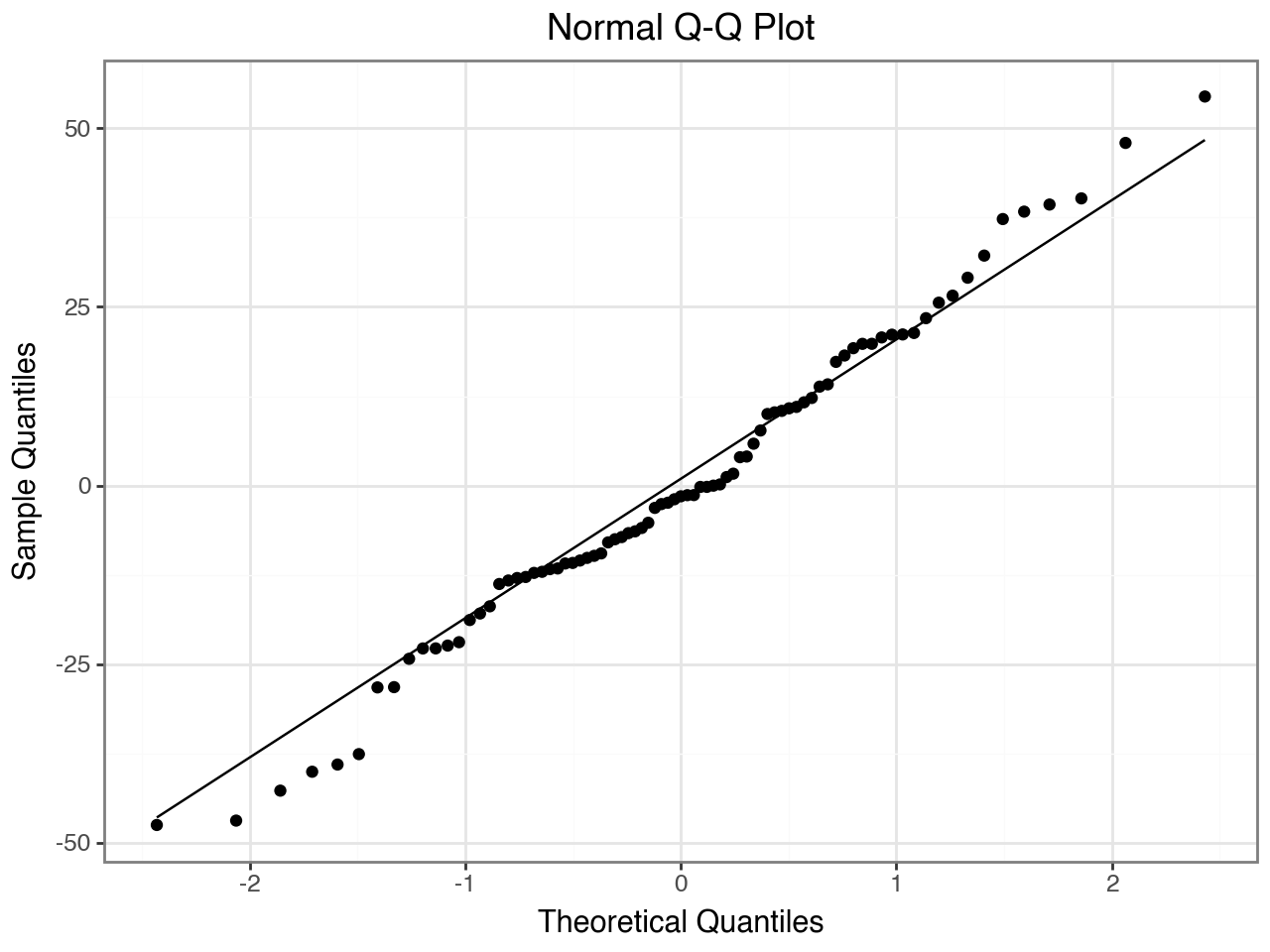
2. Q–Q plot — conditional residuals should fall approximately on the diagonal if the Gaussian assumption holds.

from interlace import hlm_resid, plot_resid

resid_df = hlm_resid(result, type="conditional")
plot_resid(resid_df, type="resid_vs_fitted")

plot_resid(resid_df, type="qq")

Summary

Register effect	Polite speech is ~19 Hz lower than informal speech (within-speaker estimate, controlling for scenario)
Subject variance	Large ICC (~0.79) — speakers differ substantially in baseline pitch, largely driven by gender
Scenario variance	Moderate ICC (~0.11) — scenario identity has a consistent but smaller effect
Diagnostics	No obvious trend in residuals vs. fitted; Q–Q plot approximately linear

The crossed structure matters here. A model with only subject random effects would conflate scenario-to-scenario variation with measurement noise, producing a larger residual variance and a wider confidence interval on is_polite. A model with only scenario random effects would ignore the strong speaker-level baseline differences, producing the opposite problem. Crossing both factors yields the most accurate decomposition.

Extensions to try

• Add gender as a fixed effect and compare to this model with a likelihood-ratio test (refit both with method="ML" first). The subject ICC should drop markedly.

• Group-level influence: hlm_influence(result, level="subject") checks whether removing any single speaker substantially changes the fixed-effect estimates.

• See Diagnostics Guide for leverage, Cook’s D, and MDFFITS plots.

• See Interpreting Model Results for a full tour of the CrossedLMEResult object.

---

Model comparison: do speakers differ in their register effect?

The baseline model assumes a single population-level register effect (−19 Hz). But do some speakers lower their pitch more than others when being polite? A random slope for is_polite by speaker tests this directly.

We compare two models using a likelihood ratio test (LRT), fitting both with method="ML" so the likelihoods are comparable:

• M0: random intercepts only — one register effect for all speakers

• M1: random intercepts + by-speaker random slope for is_polite

import scipy.stats

# Fit both with ML for LRT comparability
m0 = interlace.fit(
    "pitch_hz ~ is_polite",
    data=df,
    groups=["subject", "scenario"],
    method="ML",
)

m1 = interlace.fit(
    "pitch_hz ~ is_polite",
    data=df,
    random=[
        "(1 + is_polite | subject)",  # by-speaker random slope
        "(1 | scenario)",
    ],
    method="ML",
)

# LRT: correlated slope adds 2 parameters (slope variance + covariance)
lrt_stat = 2 * (m1.llf - m0.llf)
lrt_df   = 2
lrt_p    = scipy.stats.chi2.sf(lrt_stat, df=lrt_df)

print(f"Log-likelihoods: M0 = {m0.llf:.2f}, M1 = {m1.llf:.2f}")
print(f"LRT χ²({lrt_df}) = {lrt_stat:.3f}, p = {lrt_p:.4f}")
print(f"AIC: M0 = {m0.aic:.1f}, M1 = {m1.aic:.1f}")

Log-likelihoods: M0 = -400.28, M1 = -400.28
LRT χ²(2) = 0.002, p = 0.9990
AIC: M0 = 810.6, M1 = 814.6

/var/folders/bn/bqlvr_ys37q1c5h7jmv46z100000gp/T/ipykernel_41450/4132545678.py:11: UserWarning: boundary (singular) fit: see help(interlace.isSingular)

Since p > 0.05 (and ΔAIC = +4 favours M0), the simpler model is preferred. The data do not support meaningful between-speaker variation in the register effect — all speakers lower their pitch by roughly the same amount when speaking politely.

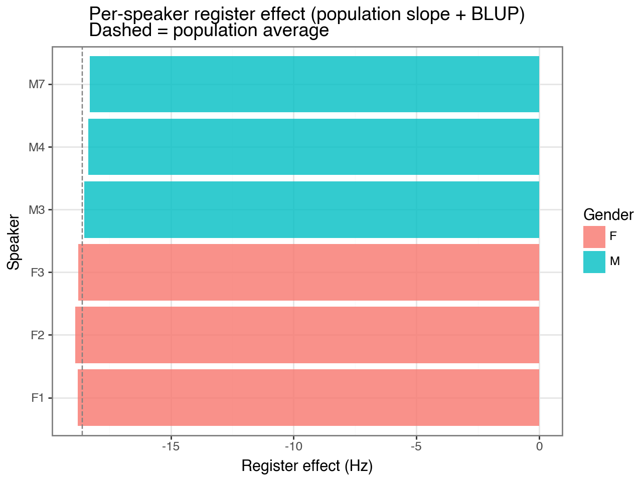
For completeness, the by-speaker random effects from M1 are shown below. The slope offsets are near zero for all speakers, confirming the LRT conclusion:

# Refit winning model with REML for final estimates
m1_reml = interlace.fit(
    "pitch_hz ~ is_polite",
    data=df,
    random=[
        "(1 + is_polite | subject)",
        "(1 | scenario)",
    ],
    # method="REML" is the default
)

# By-speaker random effects: intercept deviation + slope deviation
speaker_re = m1_reml.random_effects["subject"].copy()
speaker_re.columns = ["intercept_offset", "slope_offset"]

# Population slope + per-speaker deviation = each speaker's total register effect
pop_slope = m1_reml.fe_params["is_polite"]
speaker_re["total_register_effect"] = pop_slope + speaker_re["slope_offset"]
speaker_re = speaker_re.merge(
    df[["subject", "gender"]].drop_duplicates().set_index("subject"),
    left_index=True, right_index=True,
)
print(speaker_re[["gender", "intercept_offset", "slope_offset", "total_register_effect"]].round(2))

   gender  intercept_offset  slope_offset  total_register_effect
F1      F             48.02         -0.18                 -18.78
F2      F             77.52         -0.29                 -18.89
F3      F             42.31         -0.16                 -18.76
M3      M            -20.01          0.07                 -18.53
M4      M            -64.65          0.24                 -18.36
M7      M            -83.18          0.31                 -18.29

/var/folders/bn/bqlvr_ys37q1c5h7jmv46z100000gp/T/ipykernel_41450/1190209297.py:2: UserWarning: boundary (singular) fit: see help(interlace.isSingular)

from plotnine import geom_col, geom_errorbar, coord_flip, position_dodge

plot_df = speaker_re.reset_index().rename(columns={"index": "subject"})
plot_df["colour"] = plot_df["gender"].map({"F": "#e74c3c", "M": "#2980b9"})

(
    ggplot(plot_df, aes(x="subject", y="total_register_effect", fill="gender"))
    + geom_col(alpha=0.8)
    + geom_hline(yintercept=pop_slope, linetype="dashed", color="grey")
    + coord_flip()
    + labs(
        x="Speaker",
        y="Register effect (Hz)",
        fill="Gender",
        title="Per-speaker register effect (population slope + BLUP)\nDashed = population average",
    )
    + theme_bw()
)

---

Reporting the results

A write-up of this analysis might read:

We fitted a linear mixed-effects model predicting fundamental frequency (F0, Hz) from register (polite vs informal), with crossed random intercepts for speaker and scenario. Estimation used profiled REML (interlace v0.2.x, matching lme4::lmer).

Polite speech was produced at significantly lower pitch than informal speech (β = −18.6 Hz, SE = 5.1, p < .001). Speaker identity accounted for the largest share of variance (ICC ≈ 0.79), followed by scenario identity (ICC ≈ 0.11) and within-speaker residual variance (≈ 0.10).

A model with by-speaker random slopes for register (M1) was compared to the intercept-only model (M0) via LRT: χ²(2) = 0.00, p = .999. The slopes model was not retained; the register effect appears uniform across speakers. Residual diagnostics showed no systematic patterns.

Key values to report:

print(f"Register effect: β = {result.fe_params['is_polite']:.1f} Hz, "
      f"SE = {result.fe_bse['is_polite']:.1f}, "
      f"p = {result.fe_pvalues['is_polite']:.3f}")

total = sum(result.variance_components.values()) + result.scale
for g, v in result.variance_components.items():
    print(f"ICC ({g}): {v/total:.2f}")

---

Where to go next

• Random Slopes Guide — full guide on random slope syntax and interpretation

• Model Comparison — LRT workflow and ML vs REML guidance

• Diagnostics guide — full diagnostic suite with worked outlier example

• Interpreting model results — reading BLUPs, variance components, and fixed effects

• fit — fit() parameter reference